77-420 Online Practice Questions and Answers
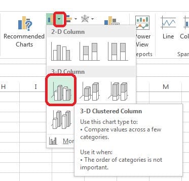
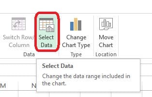
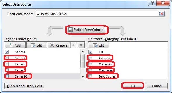
Create a chart. To the right of the data Chart 3-D Clustered Column Exclude all filtered rows Horizontal Axis Labels: "IDs" column in table Series 1: "Zero Scores" column in table.
Insert the instructor's name for column B.
Cell B5.
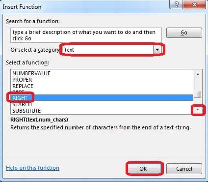
Use Function RIGHT
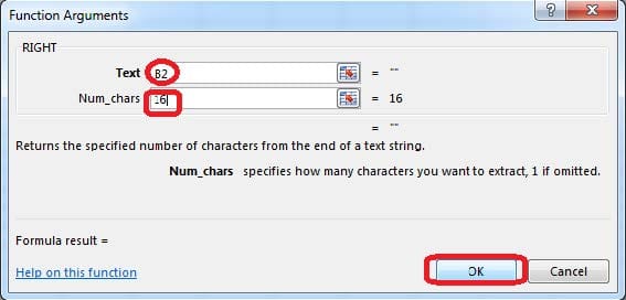
Text: B2
Absolute reference
Num_chars: "16"
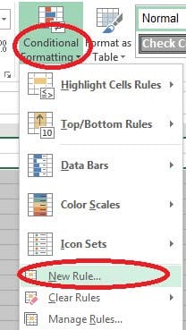
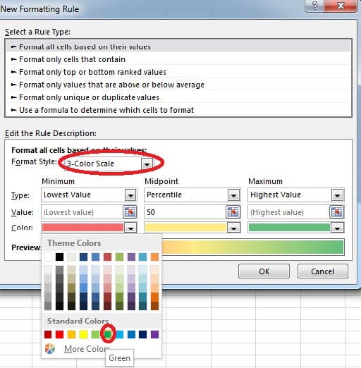
Add conditional formatting.
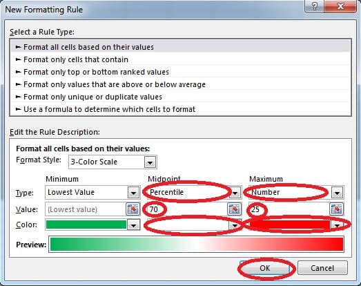
Color Scales: Green –White-Red Color Scale
Midpoint: Percentile, "70"
Maximum: Number, "25"
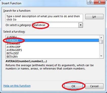
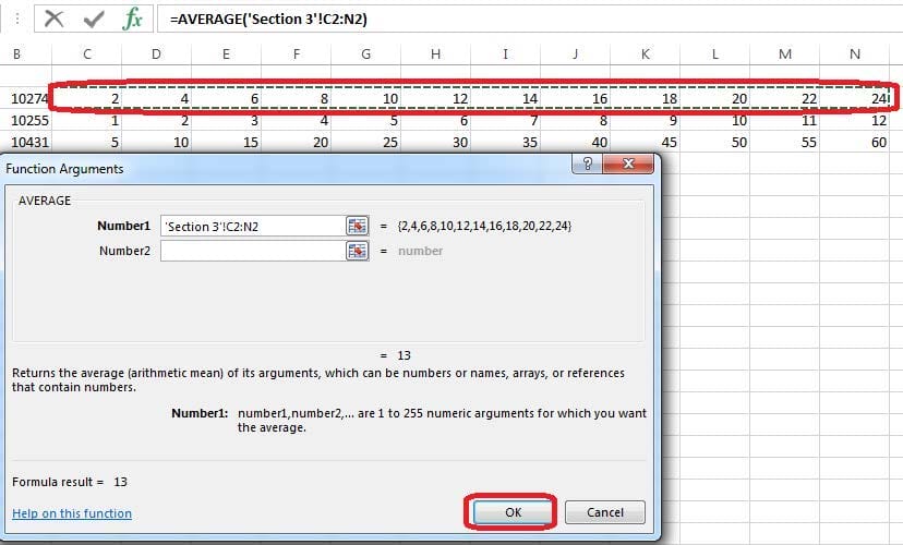
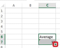
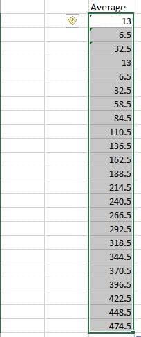
Formula. Find the average of each student's homework scores.
Cell range C7:C29
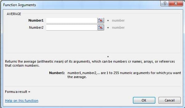
Use Function AVERAGE
Number 1: all homework for each student on "Section 3" worksheet "22-Aug 12-Dec"
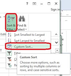
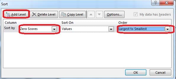
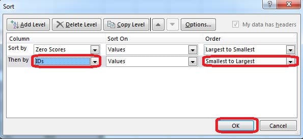
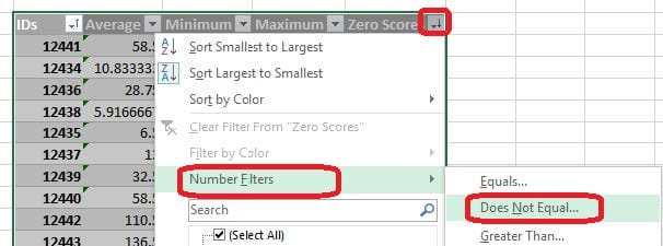
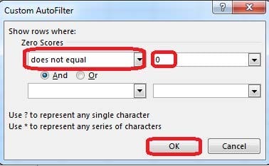
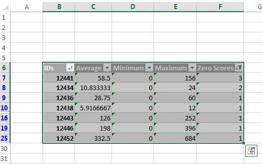
Sort and Filter. Apply a sort and a filter to the table. Cell range B6:F29 Sort Column Zero Scores Order Largest to Smallest Column IDs Order Smallest to Largest Filter Hide students ids with no zero scores.
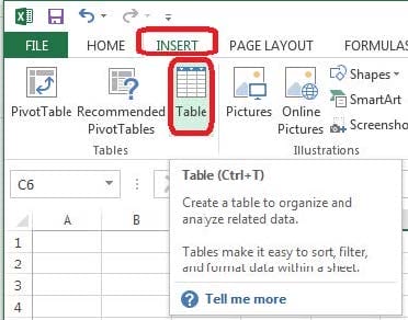
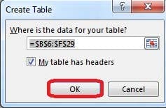
Create a table and modify the table styles. Cell range B6:F29 Table Style Medium 4 Enable the First Column Style
Add a header and the date for each of the columns (assignments) in the range.
Cell B2.
Text "Date".
Cell Range C2: S2
Text: "22-Aug, 29-Aug,
